AI Efficiency II: Pruning and Sparsity

Introduction

The pursuit of accuracy in modern AI, particularly with the advent of Large Language Models (LLMs) and vision transformers, has led us down a path of ever-increasing model scale. Branwen (2020)⁹, often cited as justification, posits that larger models, trained on more data, exhibit improved performance. And indeed, empirical evidence largely supports this – up to a point. However, this scaling comes at a steep cost, most acutely felt in memory and energy consumption.

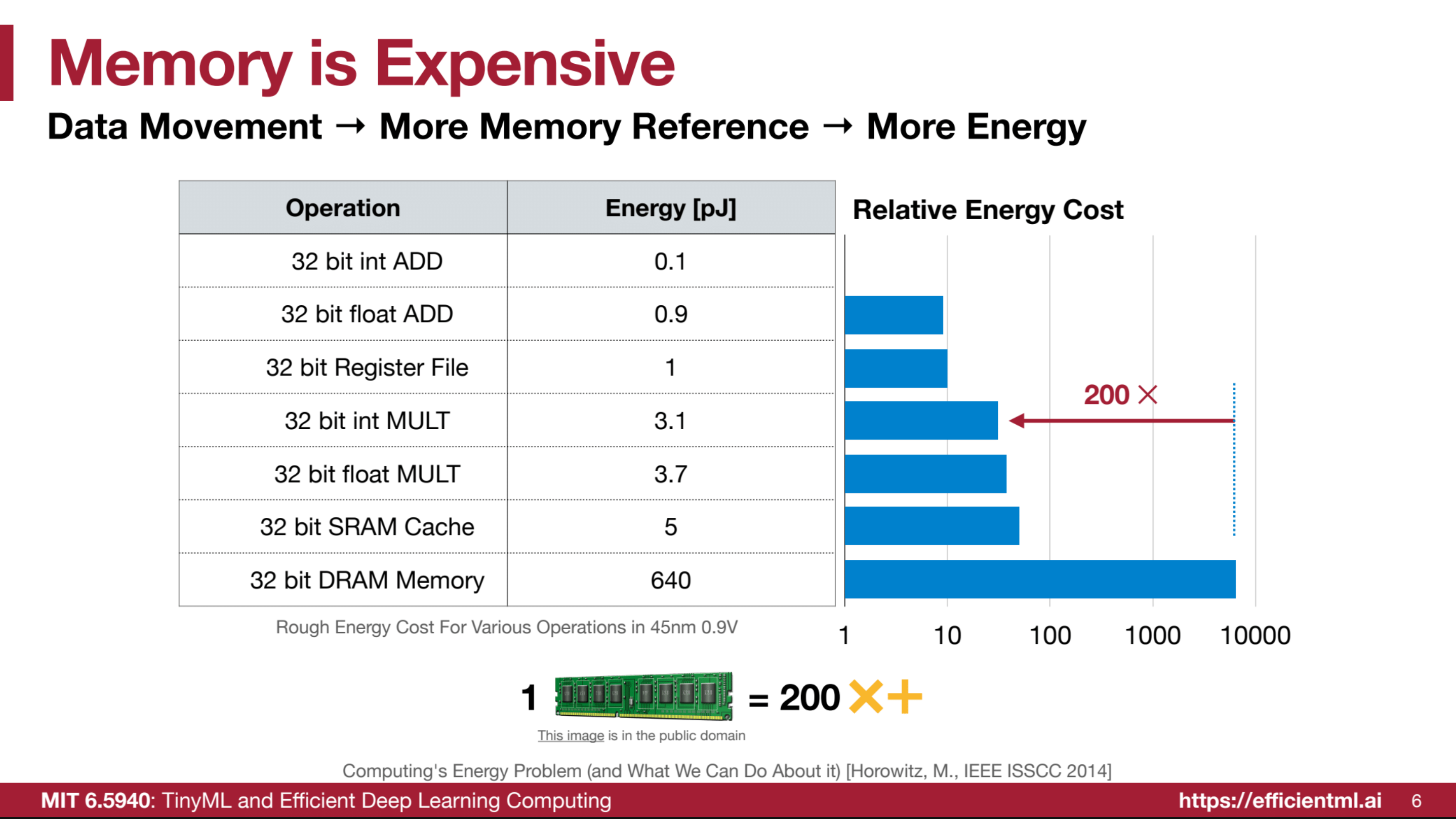
As models balloon in parameter count, so too does their memory footprint. Storing these massive models on disk is one challenge, but the real bottleneck emerges during inference and training. GPU memory, while expanding, has not kept pace with parameter proliferation. This requires constant data movement between High Bandwidth Memory (HBM) and on-chip SRAM, a process notoriously power-hungry. Horowitz (2014)¹ highlights this: energy expenditure for data movement can dwarf that of computation itself, especially across memory hierarchies. This “memory wall” (or perhaps, more accurately, “memory power draw”) threatens to make continued scaling economically and environmentally unsustainable.

_{(Image from 2)}

Thus, the imperative for efficiency becomes very important. We must explore techniques to mitigate the resource demands of these gargantuan models without sacrificing, or ideally even improving, performance. Two primary avenues present themselves: pruning and quantization. Pruning focuses on reducing the number of parameters, aiming to induce sparsity – a state where a significant proportion of model weights are zero. Quantization, conversely, reduces the precision of the remaining parameters, shrinking their storage footprint. This post will focus on the former: pruning and sparsity in neural networks.

Pruning

Neural network pruning, at its core, is about selective weight removal. Formally, we can frame it as a constrained optimization problem:

${\mathrm{argmin}}_{W_p}L(X;W_p)\text{subject to}\Vert W_p{\Vert }_0<N$

Where:

• $L$ is the loss function guiding network training.
• $\mathbf{x}$ represents the input data.
• $\mathbf{W}$ is the original, dense weight matrix.
• ${\mathbf{W}}_{\mathbf{p}}$ denotes the pruned weight matrix.
• $\Vert {\mathbf{W}}_{\mathbf{p}}{\Vert }_0$ is the ${\ell }_0$ “norm,” counting the number of non-zero parameters in ${\mathbf{W}}_{\mathbf{p}}$.
• $N$ is our target sparsity level - the maximum allowed non-zero weights.

Pruning Strategies: Neurons vs. Synapses & Granularity

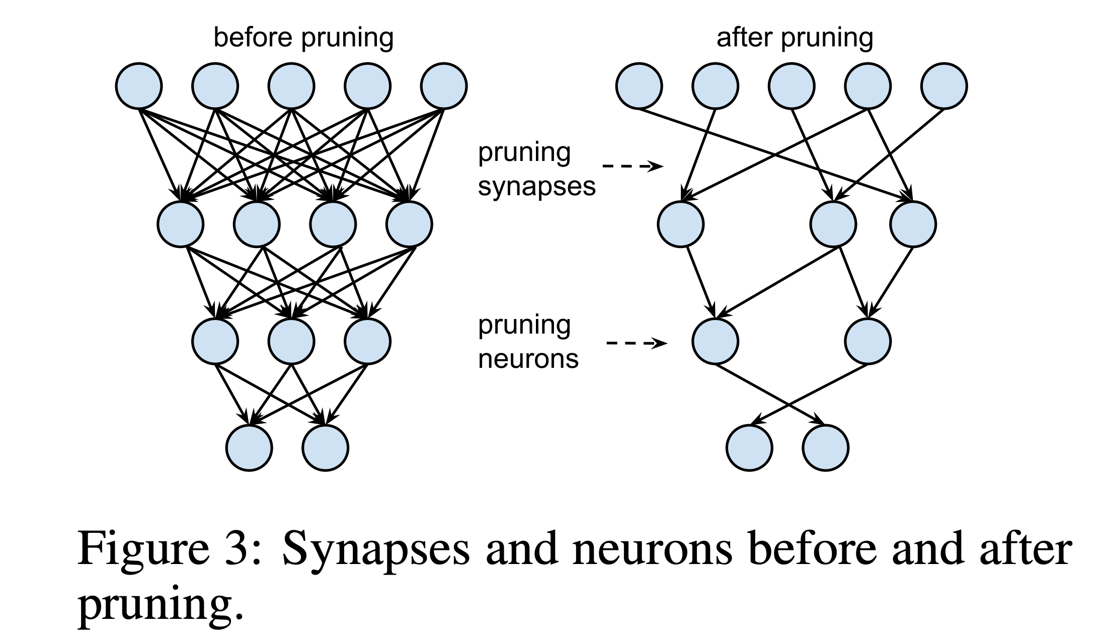
Pruning can be broadly categorized by the granularity at which weights are removed. We can prune at the level of individual synapses (connections) or entire neurons (nodes).

Neuron Pruning: This involves eliminating entire neurons, either within a layer (width pruning) or by removing layers altogether (depth pruning). The rationale is that some neurons may be redundant or contribute negligibly to the network’s overall function. Removing them simplifies the network architecture, potentially leading to faster inference and reduced memory usage. However, neuron pruning can be a more coarse-grained approach, potentially leading to larger accuracy drops if not performed judiciously.

Synapse Pruning: Synapse pruning, conversely, targets individual connections (weights) between neurons. Weights with magnitudes below a certain threshold are set to zero. This induces sparsity at a finer granularity, potentially preserving more of the network’s representational capacity compared to aggressive neuron pruning. Synapse pruning can lead to unstructured sparsity (individual weights zeroed out) or structured sparsity (patterns of zeros enforced, as discussed later).

_{(Image from 3)}

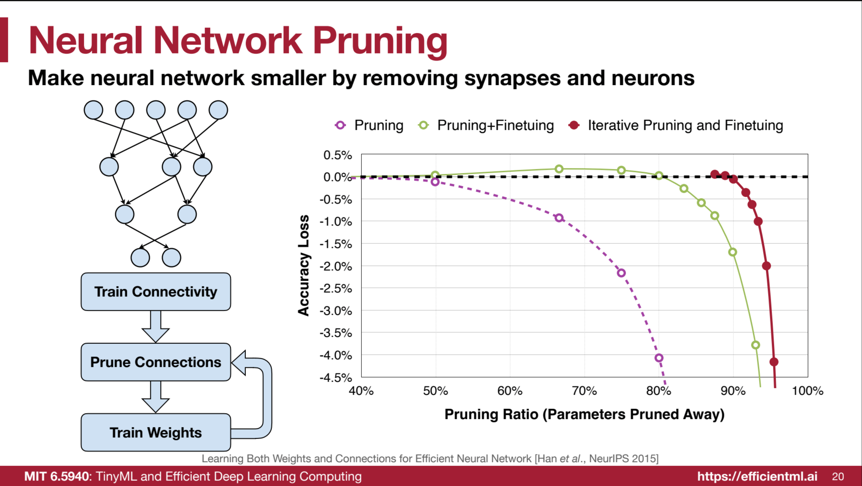
Han et al. (2015)³ demonstrated the effectiveness of iterative magnitude pruning. They trained a baseline network (AlexNet), then pruned small-magnitude weights, and crucially, fine-tuned the remaining weights. This iterative prune-and-fine-tune cycle proved highly effective.

_{(Image from 2, based on 3)}

As the figure illustrates, naive pruning (simply removing weights without retraining) leads to accuracy degradation proportional to the pruning ratio. However, by fine-tuning after each pruning step, the network recovers remarkably well. ³ showed that AlexNet could be pruned by ~80% with minimal accuracy loss, and iterative pruning could push this to ~90% sparsity. The key insight here is that fine-tuning allows the network to redistribute importance among the remaining connections, compensating for the pruned ones.

Granularities of Pruning

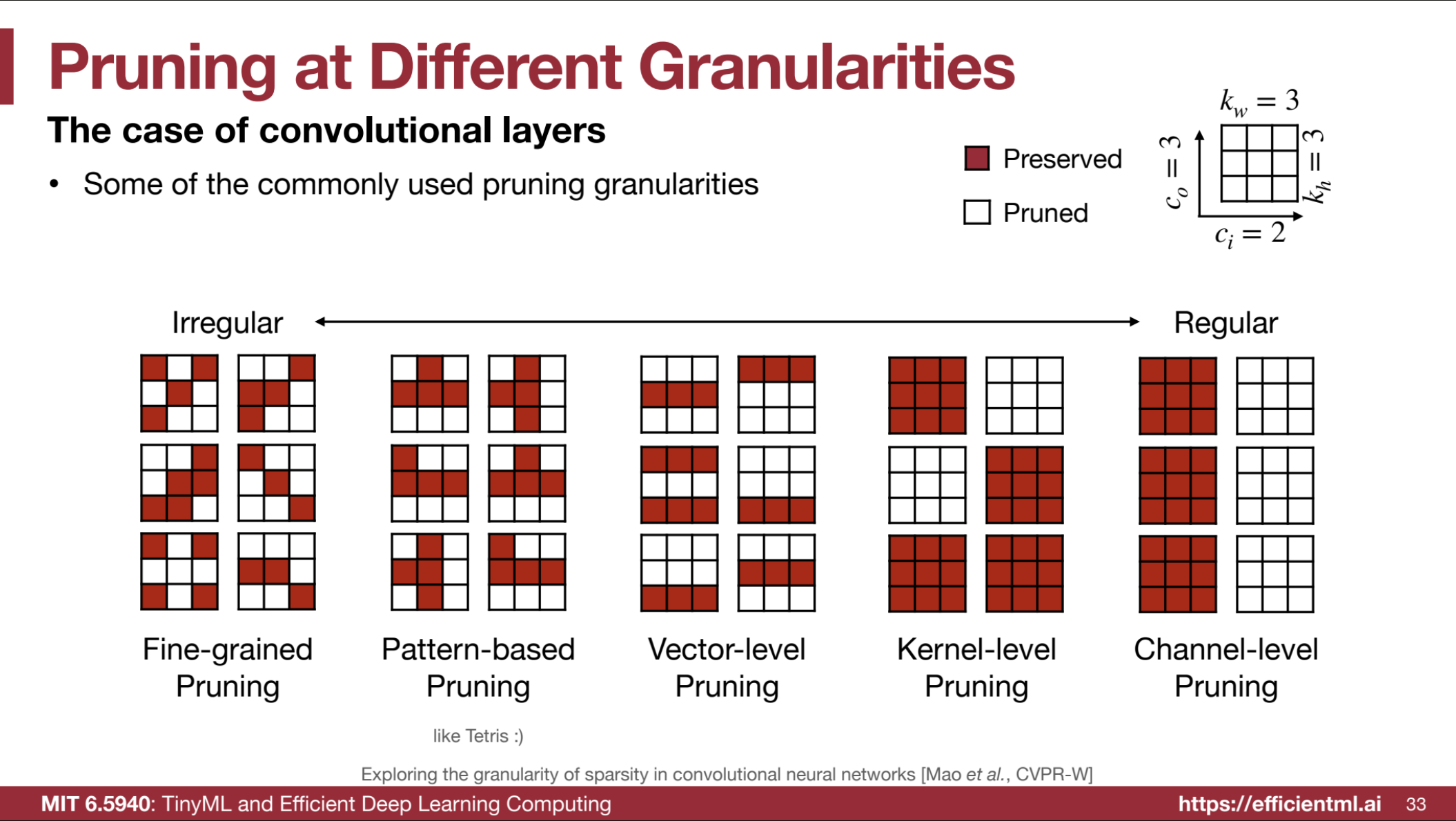
Beyond neuron vs. synapse, pruning can be further categorized by granularity, particularly relevant in Convolutional Neural Networks (CNNs). CNNs, with their kernel-based operations, offer various structural levels for pruning:

Fine-grained (Element-wise) Pruning: Individual weights within kernels or weight matrices are pruned based on some criterion (e.g., magnitude). Offers the highest flexibility and potential compression ratio, but often results in unstructured sparsity, which is less hardware-friendly on standard GPUs.

Pattern-based (N:M) Pruning: Enforces structured sparsity by requiring specific patterns of zeros within weight blocks (e.g., 2:4 sparsity, where in every block of 4 consecutive values, at least 2 must be zero). This is specifically designed to leverage hardware acceleration, such as NVIDIA’s sparse tensor cores, but may limit achievable sparsity compared to fine-grained pruning.

Vector-based (Row/Column) Pruning: Prunes entire rows or columns in weight matrices, effectively removing neurons or filters. Strikes a balance between granularity and structure.

Kernel-based Pruning: Removes entire kernels in convolutional layers. More aggressive than vector pruning, leading to simpler filters and reduced computation.

Channel-based Pruning: Specifically for CNNs, removes entire channels (feature maps). This is often considered more structurally sound for CNNs as channels represent distinct features. Channel pruning can be seen as a form of neuron pruning at the feature map level.

_{(Image from 2)}

The choice of pruning granularity involves trade-offs between compression ratio, hardware acceleration potential, and implementation complexity. Fine-grained pruning offers maximum flexibility but may not directly map to hardware speedups without specialized sparse compute units. Structured pruning, particularly pattern-based sparsity, is explicitly designed for hardware acceleration but might constrain the achievable sparsity level and require careful implementation.

Pruning in Industry: NVIDIA’s Structured Sparsity

NVIDIA’s Ampere and Hopper architectures [⁵, ⁶] have brought structured sparsity to the forefront of hardware-accelerated AI inference. Their Tensor Cores, starting from the Ampere generation, leverage 2:4 structured sparsity to achieve up to 2x throughput gains while maintaining accuracy for matrix multiplications.

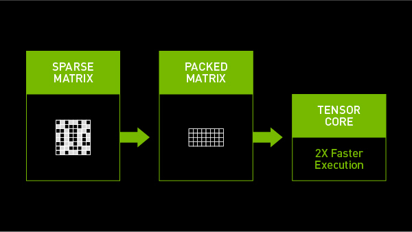
_{(Image from 4)}

Structured Sparsity: 2:4 Pattern

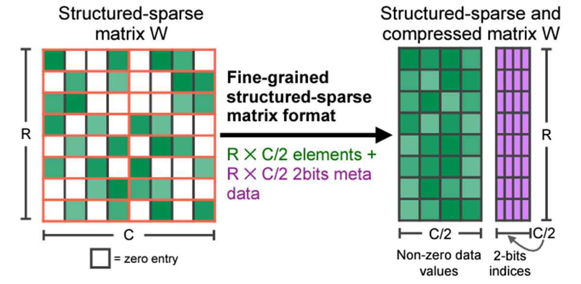
_{(Image from 5)}

NVIDIA’s sparse Tensor Cores are optimized for 2:4 sparsity. This requires that within every group of four contiguous values in a weight tensor, at least two must be zero. This enforces a 50% sparsity rate. The concept generalizes to N:M sparsity, where in a block of M values, N must be zero. During storage, only the non-zero values and associated metadata (indices indicating their original positions) are kept, leading to compression. This is primarily applicable to fully connected and convolutional layers.

The performance gain arises because Sparse Tensor Cores operate only on the non-zero values. The metadata guides the hardware to fetch only the necessary corresponding values from the dense operand in a matrix multiplication, effectively skipping computations involving zeros ⁶. For 2x sparsity, this can, ideally, halve the computation time for matrix multiplications, a core operation in deep learning.

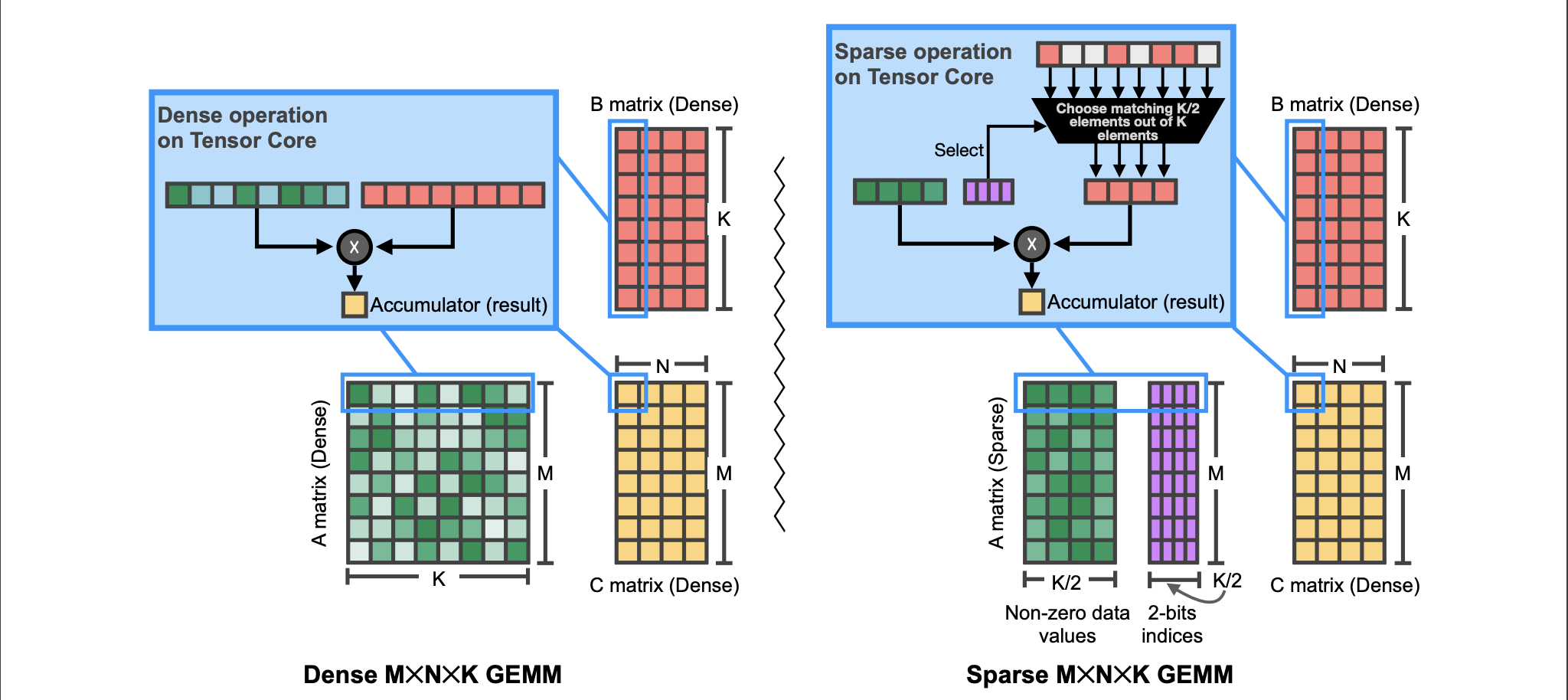
_{(Image from 7)}

Consider a GEMM (Generalized Matrix Multiply) operation: $C=A\times B$, where $A\in {\mathbb{R}}^{M\times K}$ is sparse (2:4 structured sparsity), and $B\in {\mathbb{R}}^{K\times N}$ is dense. Sparse Tensor Cores accelerate this by effectively transforming the dense GEMM into a sparse one. While the logical dimensions of $A$ remain $M\times K$, its compressed representation and the sparse hardware allow computation only on the non-zero elements of $A$ and the corresponding rows of $B$. This hardware-level optimization is a significant driver for adopting structured sparsity in practical deployments.

However, it’s crucial to note that the theoretical 2x speedup is often not fully realized in practice due to overheads like metadata processing and memory access patterns. Empirical benchmarks are essential to quantify the actual gains in specific use cases.

This hardware-level optimization is a significant driver for adopting structured sparsity in practical deployments. However, it’s crucial to note that the theoretical 2x speedup is often not fully realized in practice due to overheads like metadata processing and memory access patterns. Empirical benchmarks are essential to quantify the actual gains in specific use cases.

Pruning Criteria

The efficacy of pruning relias on identifying and removing “unimportant” weights. Various criteria exist to assess weight importance. Magnitude-based pruning is a common and straightforward approach.

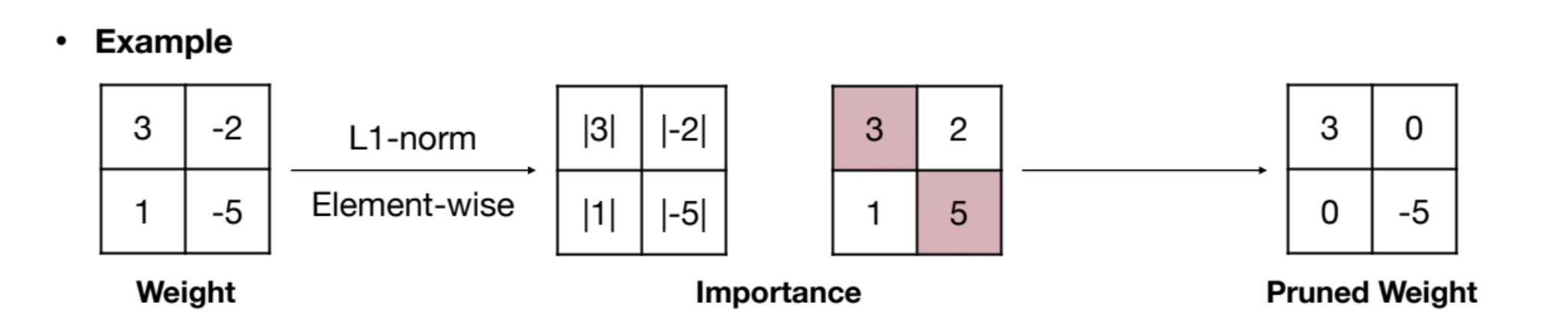
Magnitude-Based Pruning

The intuition is that weights with smaller absolute values contribute less to the network’s output and can be pruned.

Element-wise Pruning

The simplest form, where individual weights below a threshold are zeroed out.

_{(Image from 2)}

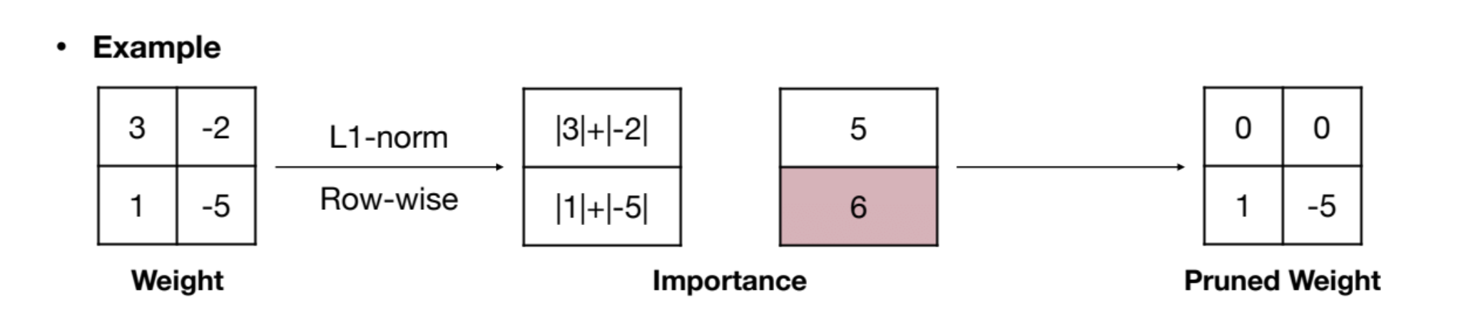
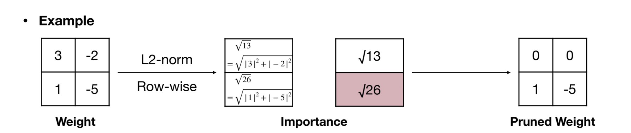
Structural Pruning with Norms

For structured pruning (e.g., row, column, kernel), norms can be used to assess the “importance” of entire structures. Common norms include $l_1$, $l_2$, and generalized $l_p$ norms.

$l_1$-norm

Importance is calculated as the sum of absolute values within a structural unit (eg: a row):

$\text{Importance}={\sum }_{i\in S}|w_i|$

where $S$ is the set of indices in the structural units.

_{(Image from 2)}

_{(Image from 2)}

Beyond Magnitude

More Sophisticated Criteria

While magnitude-based pruning is widely used due to its simplicity, it’s not necessarily the most effective criterion. More advanced methods consider:

Gradient-based Pruning

Weights with small gradients during training are considered less important. This directly relates to the weight’s contribution to loss reduction. Techniques like Optimal Brain Damage (LeCun et al., 1990¹⁰) and Optimal Brain Surgeon (Hassibi et al., 1993¹¹) fall into this category, though they can be computationally expensive for large networks.

Connection Sensitivity

Methods that attempt to directly estimate the impact of removing a connection on the network’s output. This can involve approximating the Hessian of the loss function (second-order information) to assess sensitivity. Again, computationally demanding but potentially more accurate.

Data-Driven/Activation-Based Pruning

Pruning decisions based on the actual activations observed during inference on a dataset. For instance, neurons or channels with consistently low activations might be deemed less important and pruned.

Pruning Schedules and Strategies:

One-Shot Pruning

Prune the network once, based on a chosen criterion and sparsity target, then fine-tune the remaining weights. Simple but may be suboptimal for high sparsity levels.

Iterative Pruning

Repeated cycles of pruning and fine-tuning. As demonstrated by Han et al. 3, this often yields better results, allowing the network to adapt to sparsity more effectively. Schedules can be fixed (prune by X% every Y epochs) or adaptive.

Pruning During Training

Integrate pruning directly into the training process. Regularization terms can be added to the loss function to encourage sparsity during training itself. Less common than post-training pruning but an active research area.

Dynamic Sparsity

Sparsity patterns are not fixed but change during training or even during inference. This adds complexity but could potentially offer greater flexibility and efficiency.

Practical Considerations & Open Questions

While pruning offers a promising route to AI efficiency, several practical aspects and open research questions remain:

Software Tools and Libraries

Frameworks like PyTorch and TensorFlow provide built-in modules and libraries to facilitate pruning. NVIDIA TensorRT 4 is crucial for deploying sparse models on NVIDIA hardware, optimizing for sparse tensor core utilization. However, tooling is still evolving, and seamless integration of complex pruning strategies can be challenging.

Hyperparameter Tuning for Pruning

Pruning introduces new hyperparameters: sparsity level, pruning schedule, fine-tuning epochs, pruning criterion thresholds, etc. Tuning these effectively can be non-trivial and often requires experimentation. Automated pruning hyperparameter search is an area of active research.

Model Architectures and Pruning Sensitivity

Different network architectures exhibit varying degrees of prune-friendliness. Some architectures are inherently more robust to pruning than others. Understanding architectural biases towards sparsity is crucial for effective pruning. Transformers, for instance, may respond differently to pruning compared to CNNs.

Impact on Training Time

While the goal is to reduce inference time, the pruning process itself (especially iterative pruning with fine-tuning) can add to the overall training time. Careful scheduling and efficient implementation are needed to mitigate this.

Quantization and Pruning Synergy

Pruning and quantization are often used in tandem. Applying quantization to already sparse models can further compress them and improve inference efficiency. Exploring the optimal combination and ordering of these techniques is an ongoing area of investigation.

Pruning Large Language Models (LLMs)

Pruning LLMs presents unique challenges due to their scale and the sensitivity of their performance to even small perturbations. Maintaining perplexity and generation quality after pruning is paramount. Techniques like attention head pruning, layer pruning, and specialized sparse training methods are actively being explored for LLMs.

Lottery Ticket Hypothesis

The Lottery Ticket Hypothesis (Frankle & Carbin, 2018¹²) posits that within a randomly initialized dense network, there exists a sparse subnetwork (“winning ticket”) that can be trained in isolation to achieve comparable or even better performance than the original dense network. This suggests that sparsity is not just about compression but might be fundamental to efficient learning itself. Exploring lottery tickets and related sparse initialization strategies is a promising research direction.

Evaluation Metrics Beyond Accuracy

While accuracy preservation is crucial, evaluating pruned models should also consider compression ratio (sparsity level), inference speedup (latency reduction), and energy efficiency gains. Benchmarking across these metrics provides a more holistic picture of pruning effectiveness.

Future Directions

Research continues to push the boundaries of pruning. Areas of focus include developing more robust and automated pruning criteria, exploring dynamic sparsity, designing hardware-aware pruning algorithms, and understanding the theoretical underpinnings of sparsity in deep learning.

Conclusion: Sparse Futures

Pruning and sparsity offer a critical pathway to reconcile the insatiable demands of modern AI with the constraints of computational resources and energy efficiency. While challenges remain in terms of tooling, hyperparameter optimization, and achieving consistent and predictable performance gains, the potential benefits are undeniable. As hardware support for sparsity matures and research deepens our understanding of sparse neural networks, pruning is poised to become an indispensable technique in the toolkit of any AI practitioner aiming for both performance and sustainability. The pursuit of sparsity is not just about making models smaller; it’s about sculpting more efficient and elegant intelligence.

Acknowledgements

This blog series on AI efficiency is heavily indebted to Dr. Song Han’s course on TinyML and Efficient Deep Learning Computing⁸. The references cited and the broader field of efficient deep learning are built upon the work of numerous researchers and engineers.

I would like to extend my sincere gratitude to my colleagues for their invaluable insights and assistance throughout this research: Grok-2.0 (xAI), Gemini-2.0-Flash-Thinking-Exp-01-21 (DeepMind), O1 (OpenAI).

Their contributions have been pivotal to the success of this project, and I am deeply thankful for their collaboration.

References

1. M. Horowitz, “1.1 Computing’s energy problem (and what we can do about it),” 2014 IEEE International Solid-State Circuits Conference Digest of Technical Papers (ISSCC), San Francisco, CA, USA, 2014, pp. 10-14, doi: 10.1109/ISSCC.2014.6757323. https://ieeexplore.ieee.org/document/6757323
2. EfficientML.ai Lecture 3 - Pruning and Sparsity Part I (MIT 6.5940, Fall 2024). https://www.youtube.com/watch?v=EjsB0WgIfUM
3. Han, S., Mao, H., & Dally, W. J. (2015). Learning both Weights and Connections for Efficient Neural Networks. Advances in Neural Information Processing Systems, 28. https://arxiv.org/abs/1506.02626
4. Accelerating Inference with Sparsity Using the NVIDIA Ampere Architecture and NVIDIA TensorRT. https://developer.nvidia.com/blog/accelerating-inference-with-sparsity-using-ampere-and-tensorrt/
5. How Sparsity Adds Umph to AI Inference. https://blogs.nvidia.com/blog/sparsity-ai-inference/
6. Mishra, A., Albericio Latorre, J., Pool, J., Stosic, D., Stosic, D., Venkatesh, G., Yu, C., & Micikevicius, P. (2021). Accelerating sparse deep neural networks (arXiv:2104.08378 [cs.LG]). arXiv. https://arxiv.org/abs/2104.08378
7. Accelerating Inference with Sparsity Using the NVIDIA Ampere Architecture and NVIDIA TensorRT. https://developer.nvidia.com/blog/accelerating-inference-with-sparsity-using-ampere-and-tensorrt/
8. Dr. Song Han’s course on TinyML and Efficient Deep Learning Computing. https://hanlab.mit.edu/courses/2024-fall-65940
9. Branwen, G. (2020). The Scaling Hypothesis. https://gwern.net/scaling-hypothesis
10. LeCun, Y., Denker, J., & Solla, S. (1989). Optimal brain damage. In D. Touretzky (Ed.), Advances in Neural Information Processing Systems (Vol. 2, pp. ). Morgan-Kaufmann. https://proceedings.neurips.cc/paper_files/paper/1989/file/6c9882bbac1c7093bd25041881277658-Paper.pdf
11. Hassibi, B., & Stork, D. (1992). Second order derivatives for network pruning: Optimal Brain Surgeon. In S. Hanson, J. Cowan, & C. Giles (Eds.), Advances in Neural Information Processing Systems (Vol. 5, pp. ). Morgan-Kaufmann. https://proceedings.neurips.cc/paper_files/paper/1992/file/303ed4c69846ab36c2904d3ba8573050-Paper.pdf
12. Frankle, J., & Carbin, M. (2019). The lottery ticket hypothesis: Finding sparse, trainable neural networks (arXiv:1803.03635 [cs.LG]). arXiv. https://arxiv.org/abs/1803.03635

Tags

efficiencyaigpunvidiasparsitypruningllmhardware